SMODER Tutorial 04: HBC Result Visualization

This tutorial shows how to visualize representative SMODER outputs for the human breast cancer (HBC) RNA + ADT example.

This tutorial starts from a precomputed dataset-specific SMODER output file:

spatial_decon_result.h5ad

The upstream SMODER run follows the same general idea as Tutorial 01: run SMODER on a dataset to produce a result file, then use the result file for downstream reconstruction and visualization.

What is `spatial_decon_result.h5ad`?

In SMODER, each dataset produces its own result file, conventionally named:

spatial_decon_result.h5ad

The HBC result file is different from the Mousebrain and simulated human melanoma result files, even though the filename is the same.

For the HBC RNA + ADT example, the result file should contain:

adata.obsm["spatial"]
adata.obsm["cell_type_proportions"]
adata.obsm["embedding"]
adata.obsm["rna_encoder"]
adata.obsm["adt_encoder"]

Load the SMODER result

from pathlib import Path
import scanpy as sc

spatial_result = Path("path/to/HBC/spatial_decon_result.h5ad")
adata = sc.read_h5ad(spatial_result)

print(adata)
print(adata.obsm.keys())

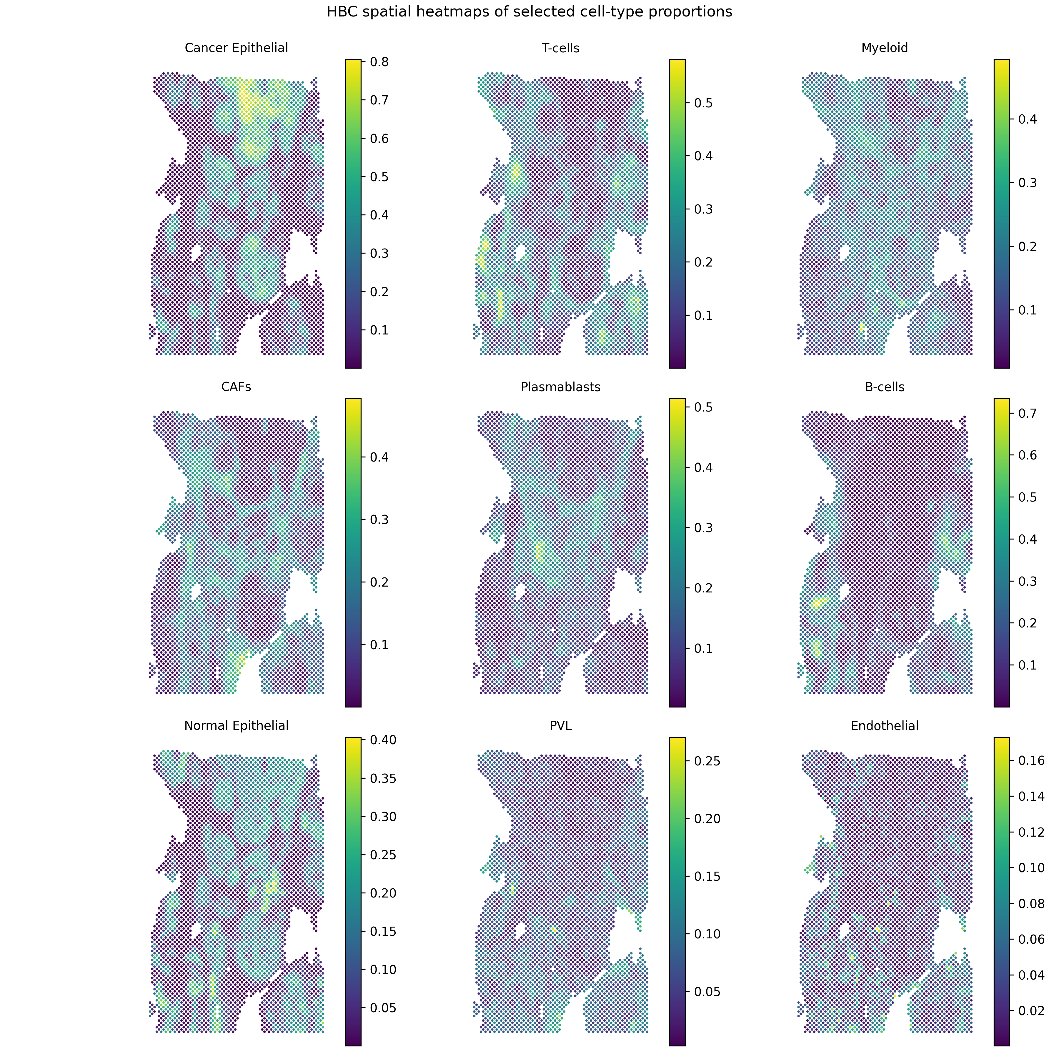
Plot cell-type proportion heatmaps

The inferred cell-type proportions are stored in:

adata.obsm["cell_type_proportions"]

For the HBC example, the first 8 columns of adata.obs are metadata, and cell-type names start from:

adata.obs.columns[8:]

Plot a compact panel of HBC cell-type proportion heatmaps:

from smoder.visualization import plot_cell_type_proportion_panel

plot_cell_type_proportion_panel(
    adata,
    out_path="hbc_cell_type_proportion_top9.png",
    obsm_key="cell_type_proportions",
    obs_start_col=8,
    top_n=9,
    ncols=3,
    title="HBC spatial heatmaps of selected cell-type proportions",
)

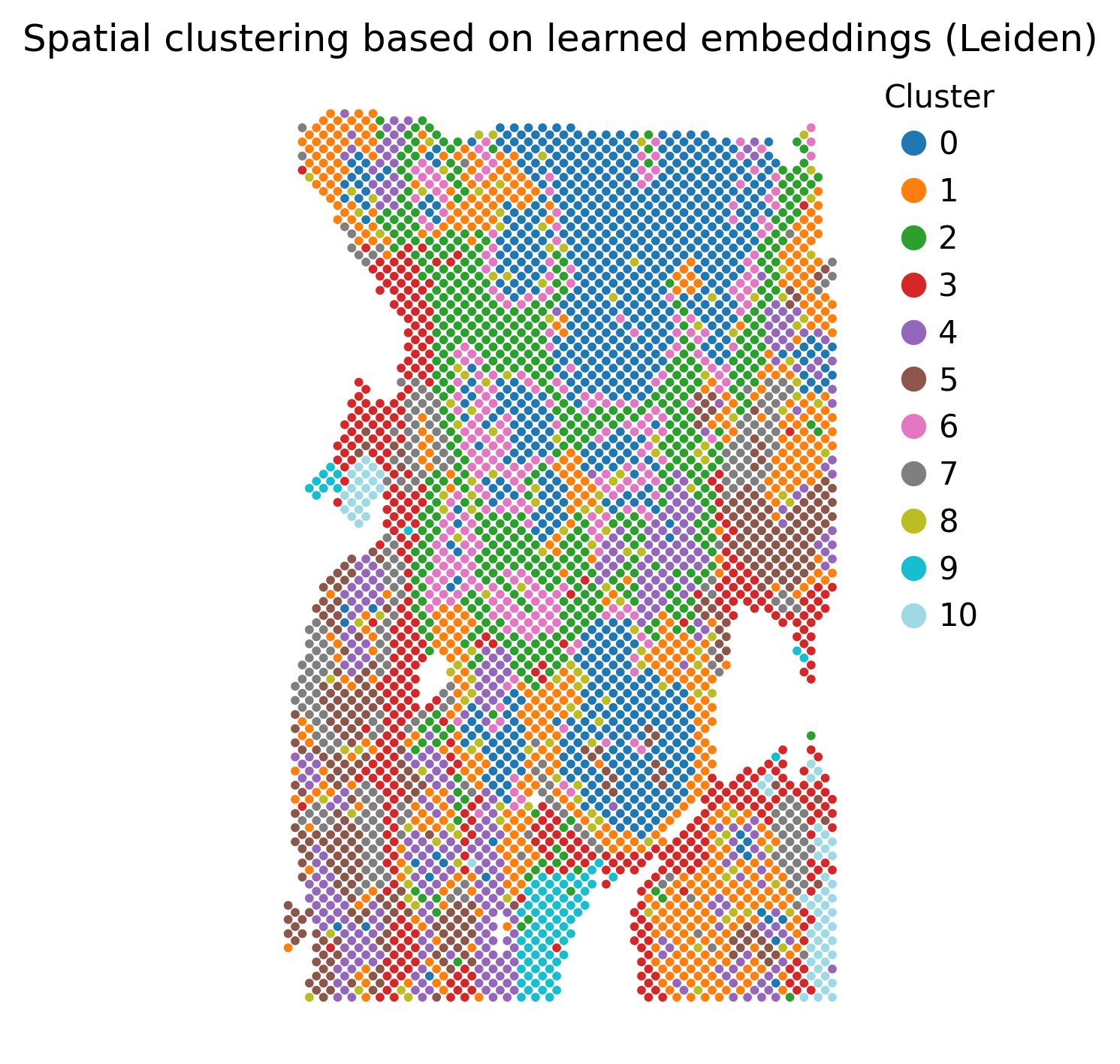
Plot spatial clusters from learned embeddings

The learned SMODER embedding is stored in:

adata.obsm["embedding"]

Cluster this embedding and visualize the cluster labels spatially:

from smoder.visualization import plot_embedding_spatial_clustering

clustered = plot_embedding_spatial_clustering(
    adata,
    out_path="hbc_embedding_spatial_clustering.png",
    embedding_key="embedding",
    method="leiden",
    resolution=0.6,
    n_neighbors=15,
)

Reconstruct denoised RNA marker expression

The RNA encoder representation is stored in:

adata.obsm["rna_encoder"]

Use omics_reconstruct to reconstruct selected RNA marker genes:

from smoder.postprocessing import omics_reconstruct

rna_recon = omics_reconstruct(
    omics_type="RNA",
    expr_path="path/to/HBC_RNA.h5ad",
    spatial_path="path/to/HBC/spatial_decon_result.h5ad",
    target_genes=["EPCAM", "KRT8", "COL1A1", "PECAM1"],
    encoder_key="rna_encoder",
    hidden_dim=256,
    n_layers=3,
    epochs=500,
    lr=1e-4,
    patience=100,
    save_path="RNA_recon.h5ad",
)

Plot the reconstructed RNA heatmaps:

from smoder.visualization import plot_reconstruction_heatmaps

plot_reconstruction_heatmaps(
    rna_recon,
    out_dir="figures",
    prefix="hbc_rna",
    title_prefix="HBC denoised RNA expression",
)

Reconstruct denoised ADT marker signals

For ADT or protein marker signals, use:

omics_type="ADT"
encoder_key="adt_encoder"

Run ADT reconstruction:

adt_recon = omics_reconstruct(
    omics_type="ADT",
    expr_path="path/to/HBC_ADT.h5ad",
    spatial_path="path/to/HBC/spatial_decon_result.h5ad",
    target_genes=["KRT5.1", "CD68.1", "CD8A.1", "HLA-DRA"],
    encoder_key="adt_encoder",
    hidden_dim=256,
    n_layers=3,
    epochs=500,
    lr=1e-4,
    patience=100,
    do_preprocess=False,
    save_path="ADT_recon.h5ad",
)

Plot the reconstructed ADT heatmaps:

plot_reconstruction_heatmaps(
    adt_recon,
    out_dir="figures",
    prefix="hbc_adt",
    title_prefix="HBC denoised ADT signal",
)

Complete plotting script

The repository provides plotting and reconstruction scripts following this workflow:

scripts/run_hbc_reconstruction_for_docs.py
scripts/plot_hbc_results_for_docs.py

You can adapt the input path variables at the top of these scripts to your own data locations.

Representative results

Cell-type proportion heatmaps

../_images/hbc_cell_type_proportion_top9.png

Spatial clustering from learned embeddings

../_images/hbc_embedding_spatial_clustering.png

Denoised RNA marker heatmaps

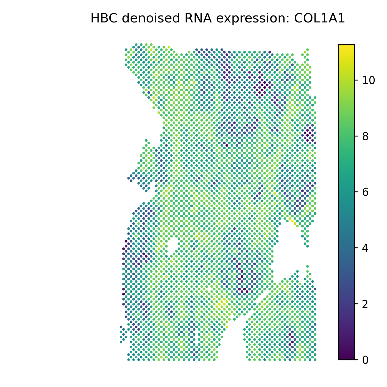
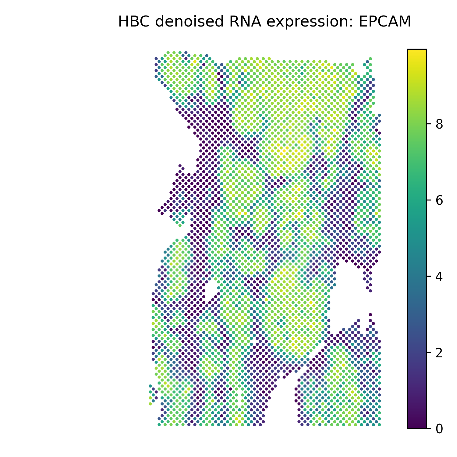
COL1A1	EPCAM
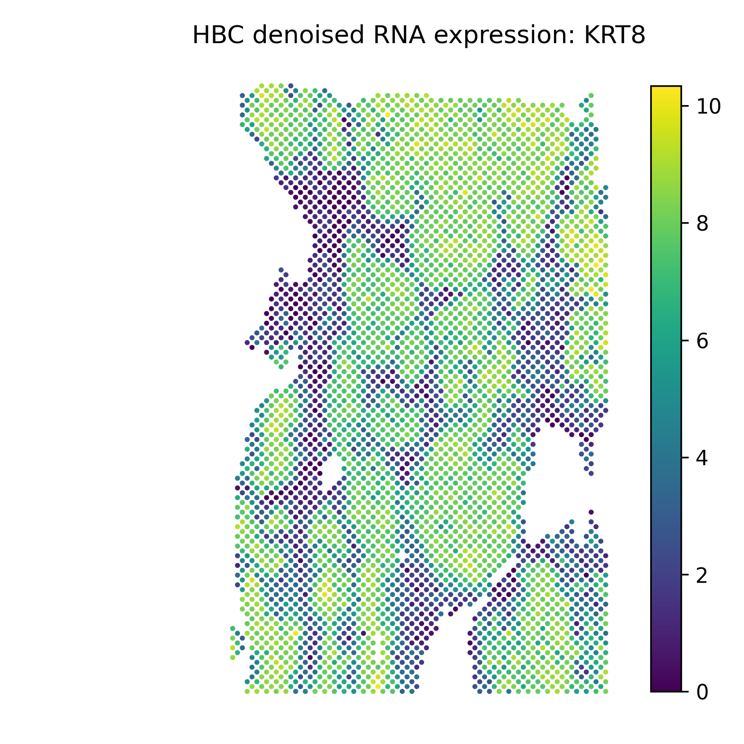
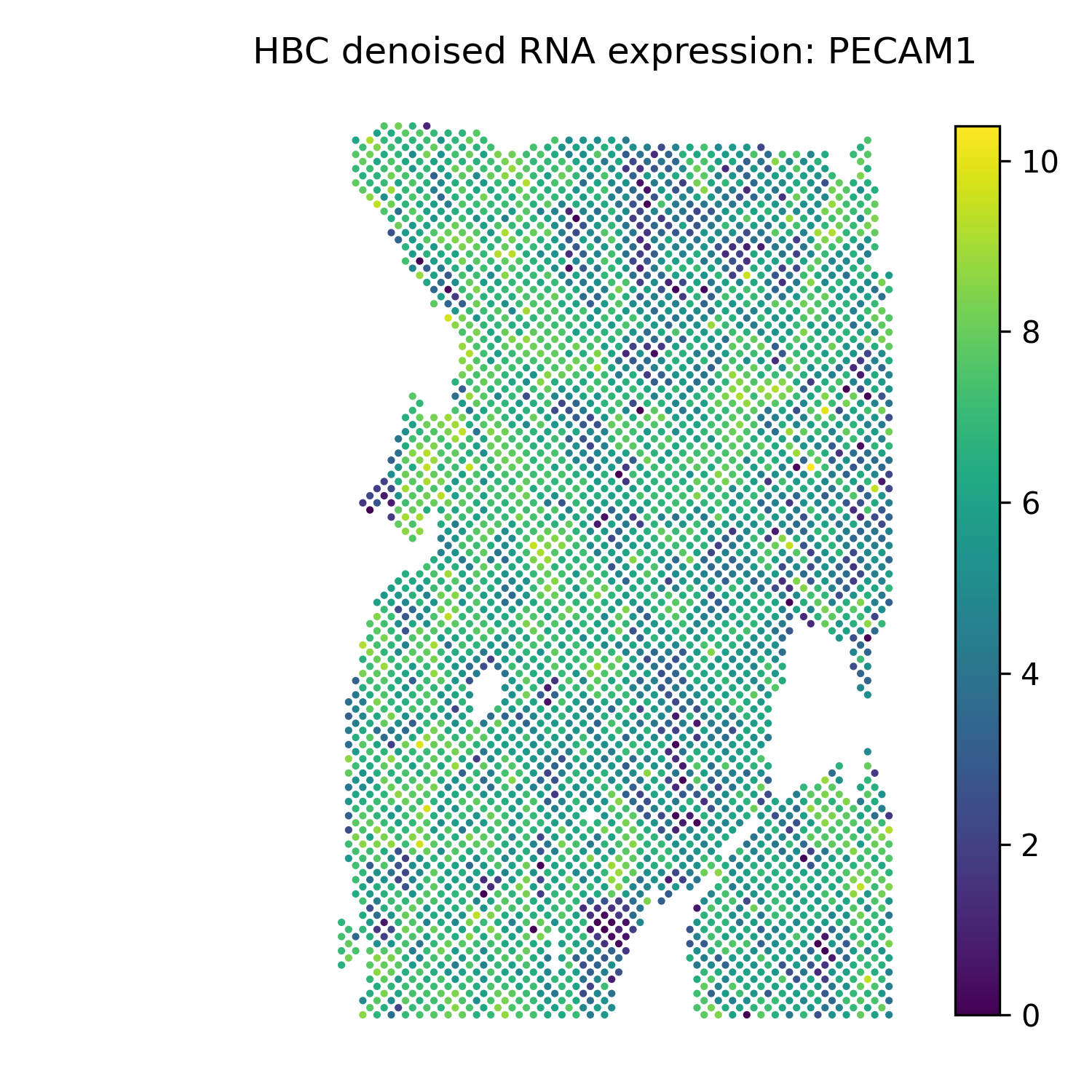
KRT8	PECAM1

Denoised ADT marker heatmaps

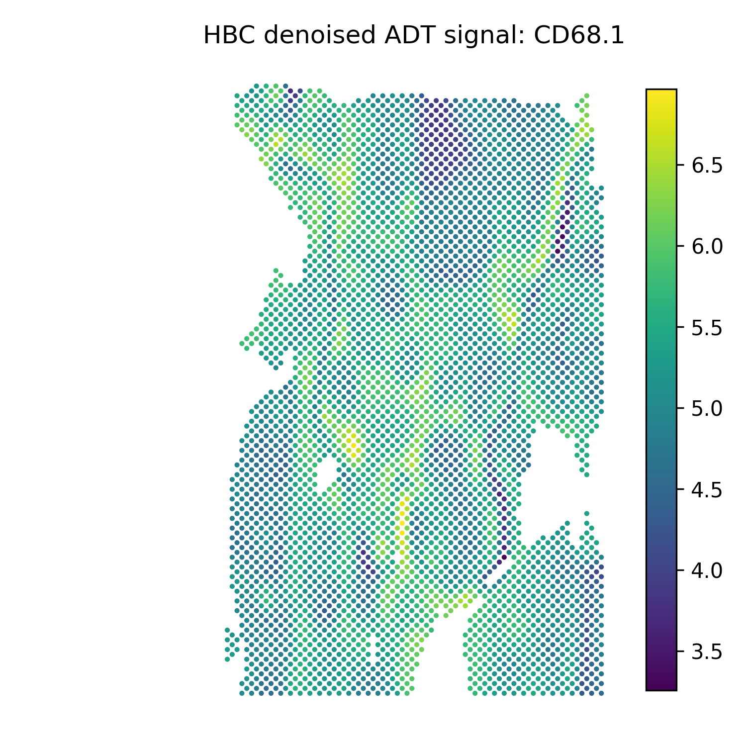
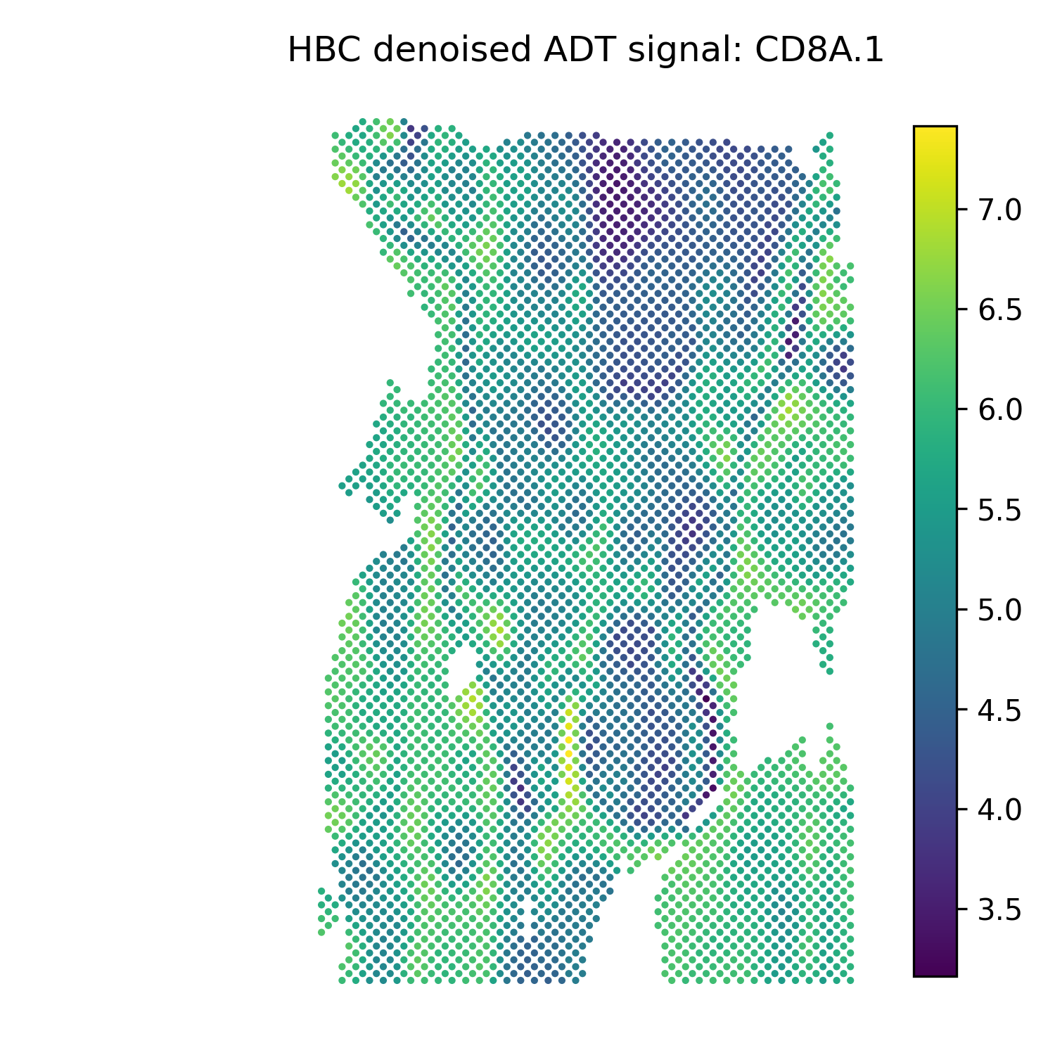
CD68.1	CD8A.1
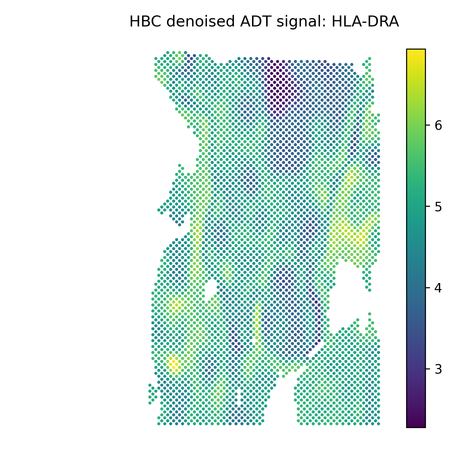
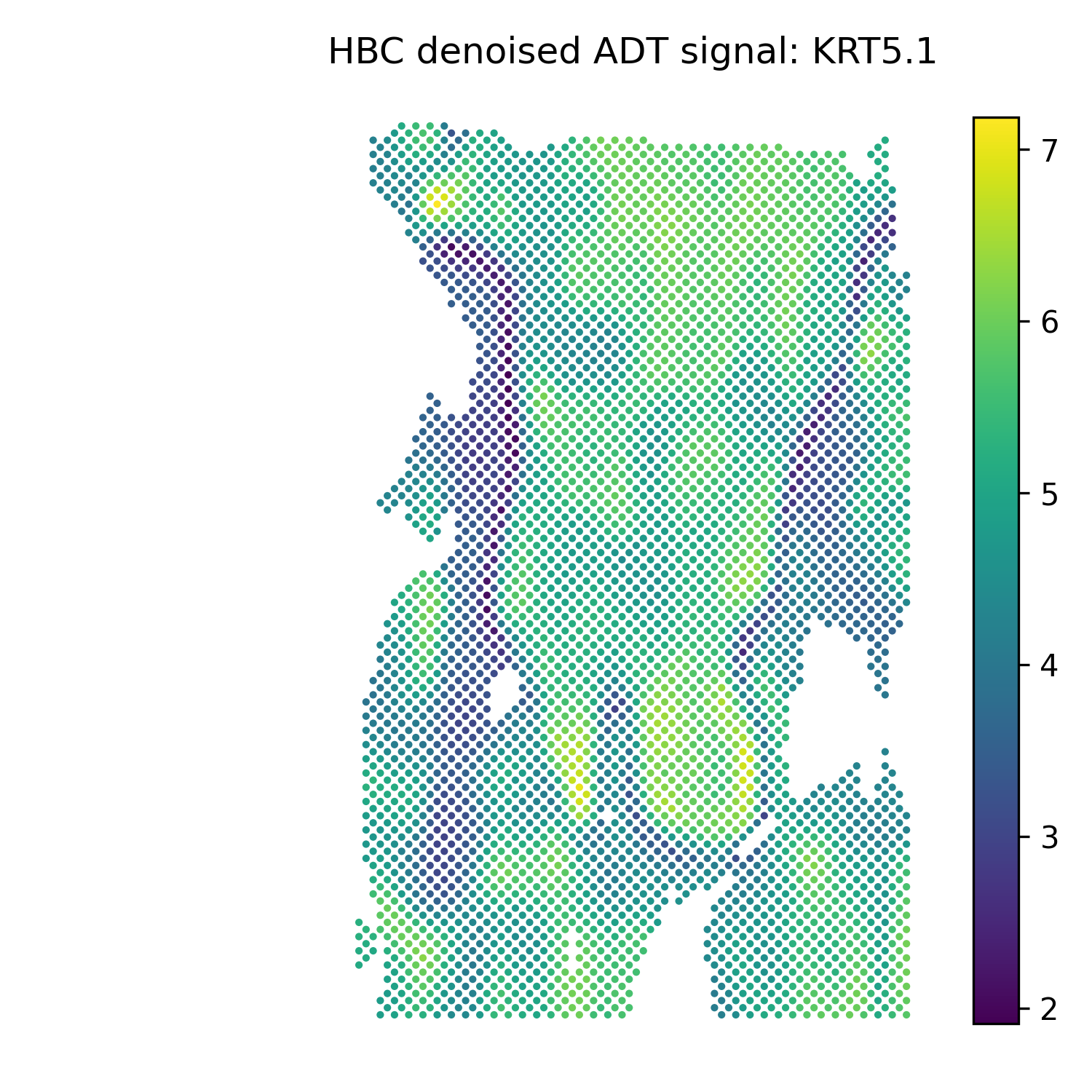
HLA-DRA	KRT5.1