SMODER Tutorial 02: Mouse Brain H3K27ac Result Visualization

This tutorial shows how to visualize representative SMODER outputs for the mouse brain RNA + H3K27ac peak example.

This tutorial continues from SMODER Tutorial 01: Mouse Brain H3K27ac Quick Start. In Tutorial 01, SMODER is run on the Mousebrain H3K27ac dataset and generates the main result file:

spatial_decon_result.h5ad

Here, we use this SMODER output file to generate downstream result visualizations.

What is `spatial_decon_result.h5ad`?

In SMODER, each dataset produces its own result file, conventionally named:

spatial_decon_result.h5ad

The same filename may appear in different output folders, but each file corresponds to a different dataset or run.

For the Mousebrain H3K27ac example, the file should contain:

adata.obsm["spatial"]
adata.obsm["cell_type_proportions"]
adata.obsm["embedding"]
adata.obsm["rna_encoder"]
adata.obsm["peak_encoder"]

These fields are used for spatial visualization, embedding-based clustering, and denoised signal reconstruction.

Load the SMODER result

from pathlib import Path
import scanpy as sc

spatial_result = Path("path/to/mousebrain_H3K27ac/spatial_decon_result.h5ad")
adata = sc.read_h5ad(spatial_result)

print(adata)
print(adata.obsm.keys())

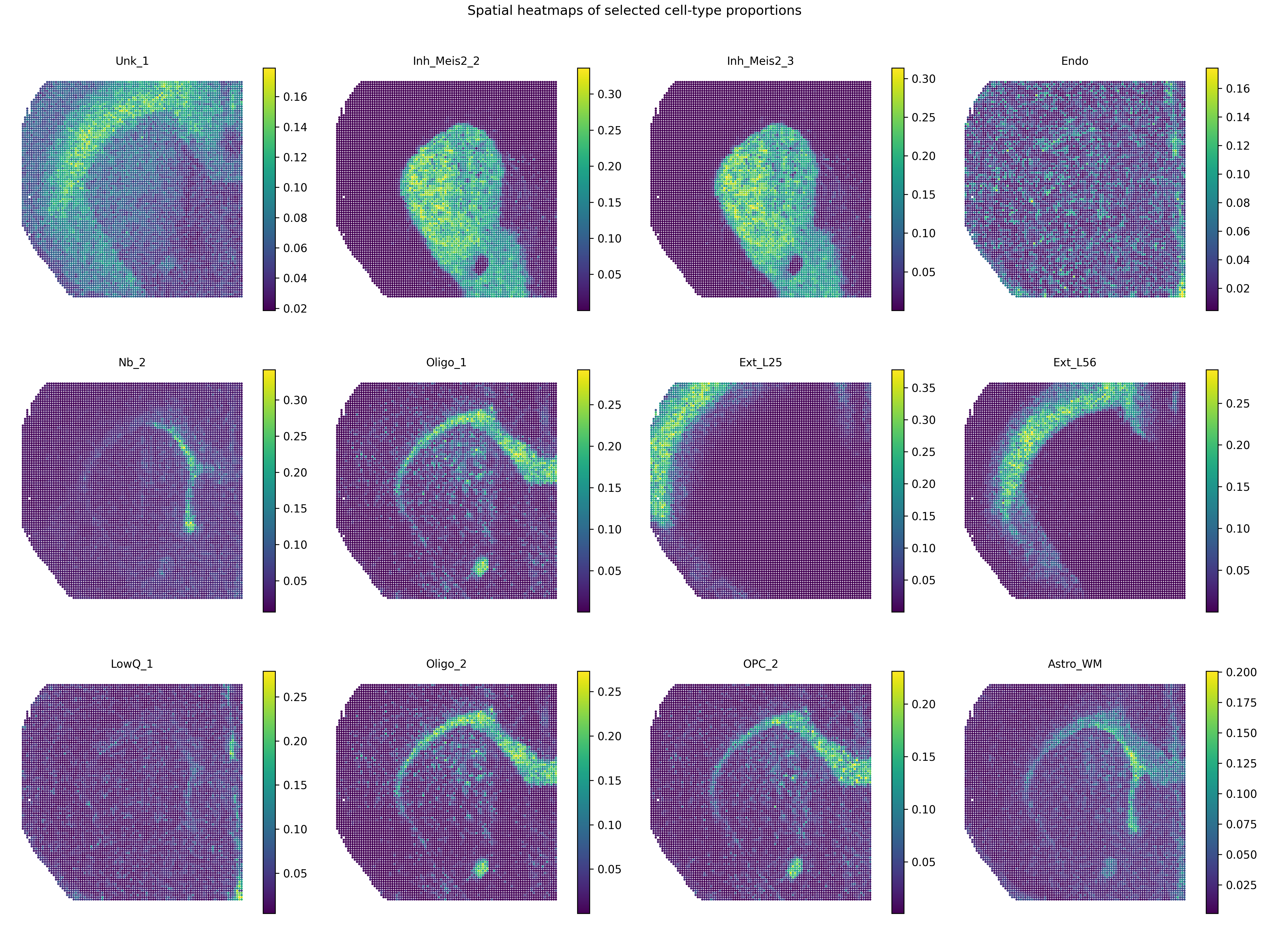
Plot cell-type proportion heatmaps

The inferred cell-type proportions are stored in:

adata.obsm["cell_type_proportions"]

The cell-type names are usually stored in adata.obs after metadata columns.

For the Mousebrain H3K27ac example, the first 9 columns of adata.obs are metadata, and cell-type names start from:

adata.obs.columns[9:]

A compact panel of cell-type proportion heatmaps can be generated by:

from smoder.visualization import plot_cell_type_proportion_panel

plot_cell_type_proportion_panel(
    adata,
    out_path="mousebrain_cell_type_proportion_top12.png",
    obsm_key="cell_type_proportions",
    obs_start_col=9,
    top_n=12,
    ncols=4,
    title="Spatial heatmaps of selected cell-type proportions",
)

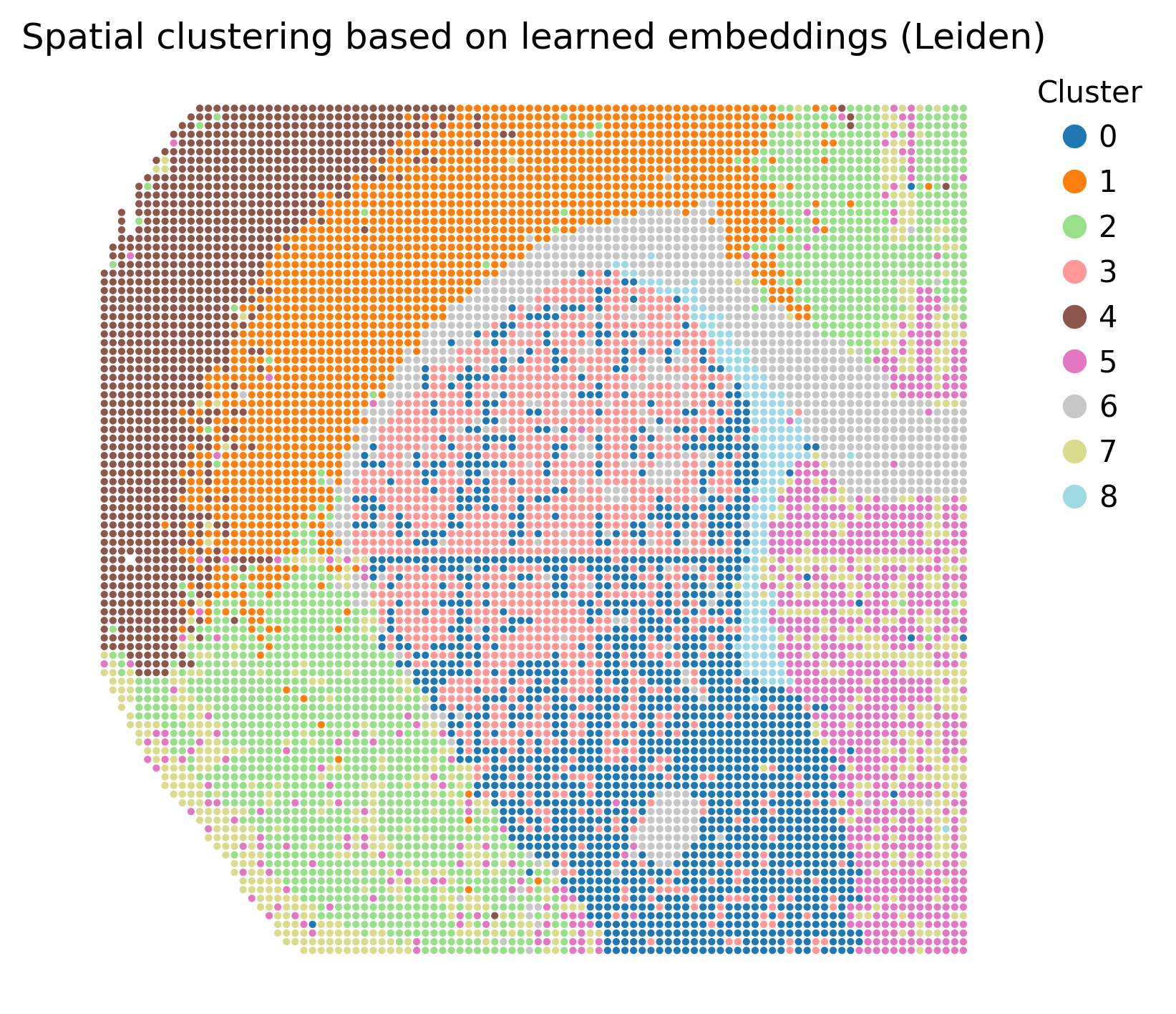
Plot spatial clusters from learned embeddings

The learned SMODER embedding is stored in:

adata.obsm["embedding"]

We can cluster this embedding and visualize the cluster labels spatially:

from smoder.visualization import plot_embedding_spatial_clustering

clustered = plot_embedding_spatial_clustering(
    adata,
    out_path="mousebrain_embedding_spatial_clustering.png",
    embedding_key="embedding",
    method="leiden",
    resolution=0.6,
    n_neighbors=15,
)

The resulting cluster labels are stored in:

clustered.obs["smoder_cluster"]

Reconstruct denoised RNA marker expression

SMODER stores RNA encoder representations in:

adata.obsm["rna_encoder"]

The function omics_reconstruct can reconstruct selected RNA marker genes from the trained SMODER representation.

from smoder.postprocessing import omics_reconstruct

rna_recon = omics_reconstruct(
    omics_type="RNA",
    expr_path="path/to/RNA.h5ad",
    spatial_path="path/to/mousebrain_H3K27ac/spatial_decon_result.h5ad",
    target_genes=["Penk", "Ppp1r1b", "Sez6l", "Gng2"],
    encoder_key="rna_encoder",
    hidden_dim=256,
    n_layers=3,
    epochs=500,
    lr=1e-4,
    patience=100,
    save_path="RNA_recon.h5ad",
)

The reconstructed values are stored in rna_recon.X.

Then plot spatial heatmaps of the reconstructed RNA markers:

from smoder.visualization import plot_reconstruction_heatmaps

plot_reconstruction_heatmaps(
    rna_recon,
    out_dir="figures",
    prefix="mousebrain_rna",
    title_prefix="Denoised RNA expression",
)

Reconstruct denoised gene-level epigenomic signals

The second modality in this example is H3K27ac peak data. For gene-level denoised visualization, use a gene-level epigenomic target matrix and the SMODER peak encoder representation:

adata.obsm["peak_encoder"]

Run reconstruction with omics_type="EPIGENOMICS":

epi_recon = omics_reconstruct(
    omics_type="EPIGENOMICS",
    expr_path="path/to/gene_level_epigenomic_signal.h5ad",
    spatial_path="path/to/mousebrain_H3K27ac/spatial_decon_result.h5ad",
    target_genes=["Penk", "Ppp1r1b", "Sez6l", "Gng2"],
    encoder_key="peak_encoder",
    hidden_dim=256,
    n_layers=3,
    epochs=500,
    lr=1e-4,
    patience=100,
    spatial_k=12,
    do_preprocess=True,
    save_path="epigenomics_recon.h5ad",
)

Then plot heatmaps of reconstructed gene-level epigenomic signals:

plot_reconstruction_heatmaps(
    epi_recon,
    out_dir="figures",
    prefix="mousebrain_epigenomics",
    title_prefix="Denoised gene-level epigenomic signal",
)

Complete plotting script

The repository also provides a plotting script that follows the same logic:

scripts/plot_mousebrain_h3k27ac_results_for_docs.py

In practice, you can adapt the path variables at the top of this script to your own local data locations.

Representative results

Cell-type proportion heatmaps

../_images/mousebrain_cell_type_proportion_top12.png

Spatial clustering from learned embeddings

../_images/mousebrain_embedding_spatial_clustering.png

Denoised RNA marker heatmaps

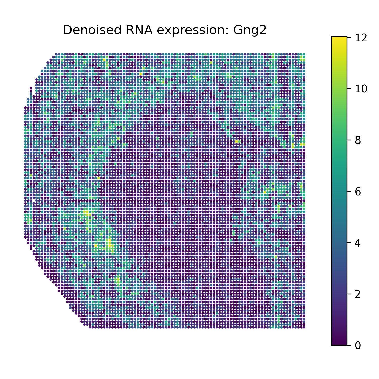
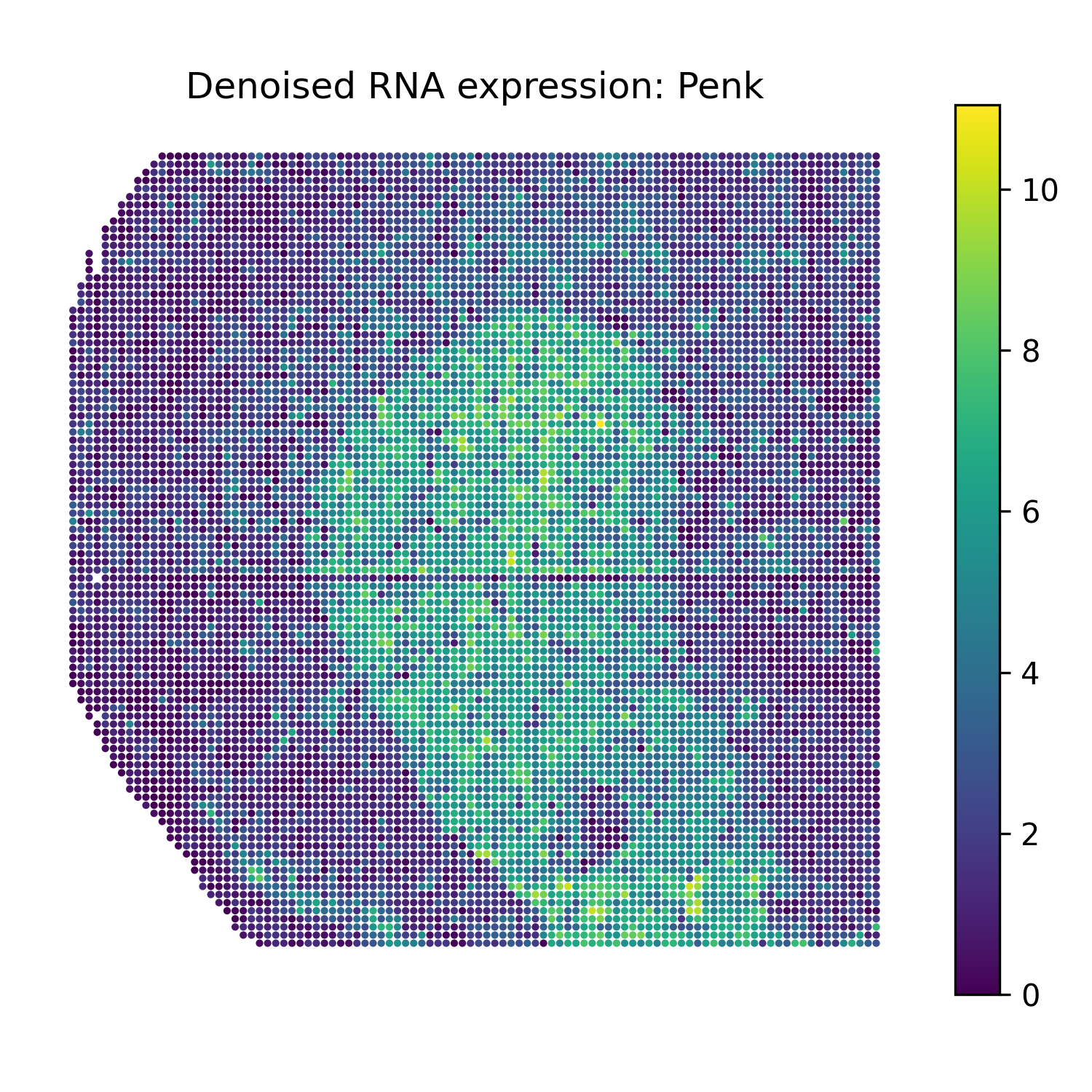
Gng2	Penk
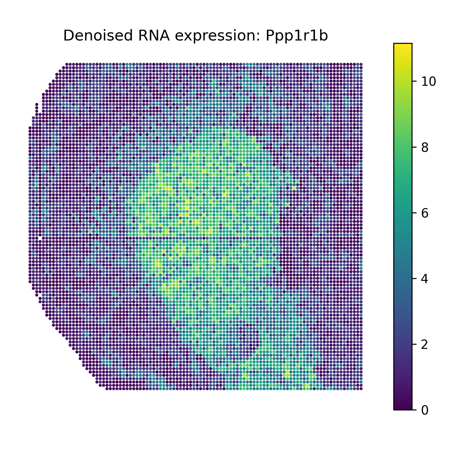
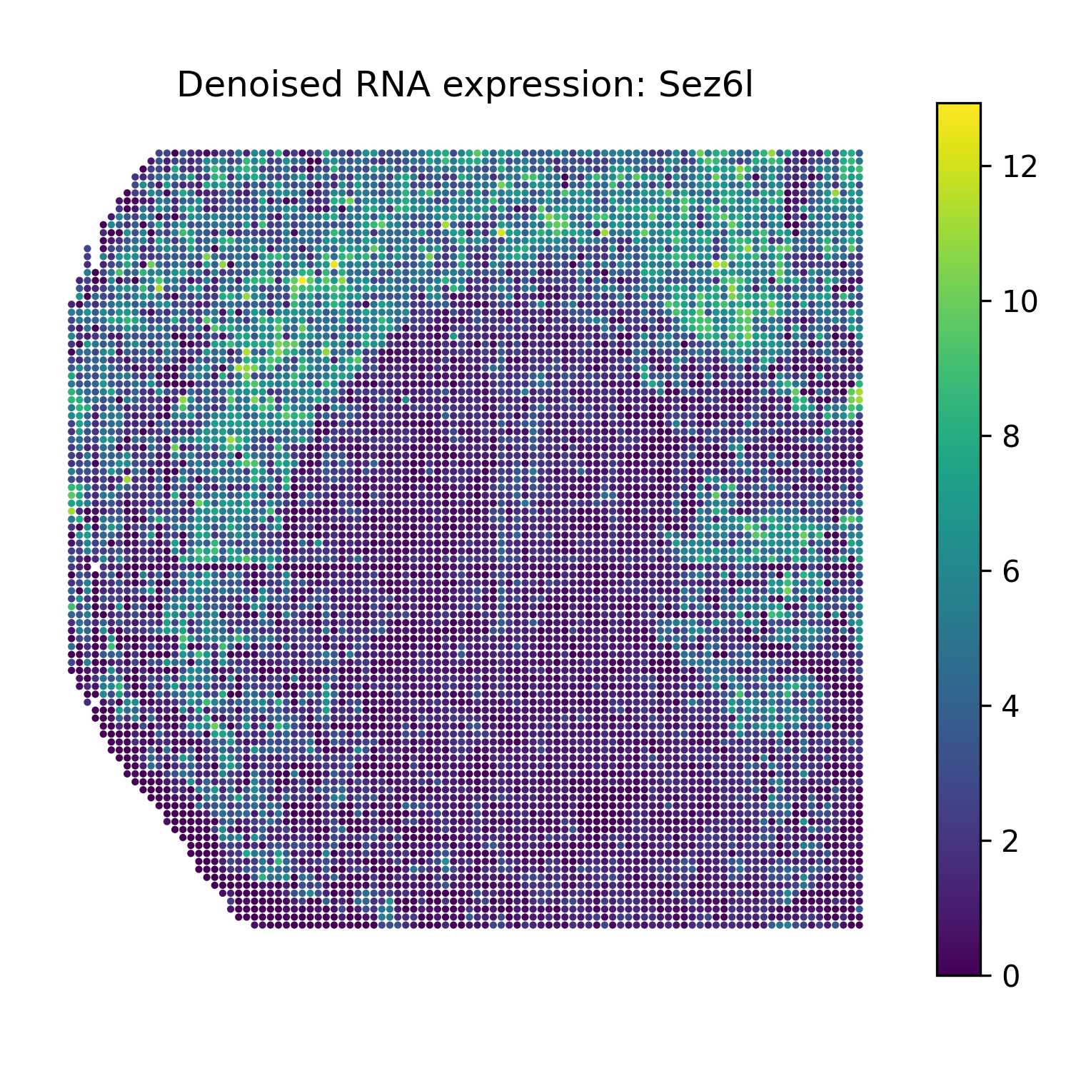
Ppp1r1b	Sez6l

Denoised gene-level epigenomic signal heatmaps

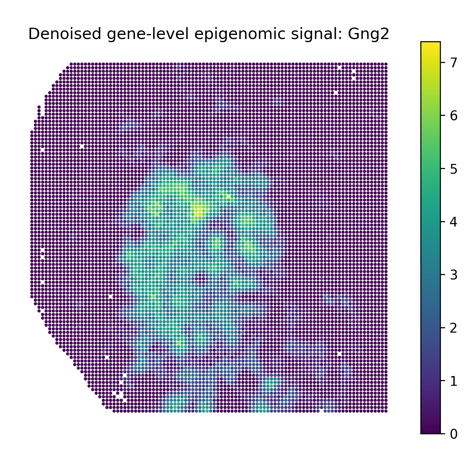
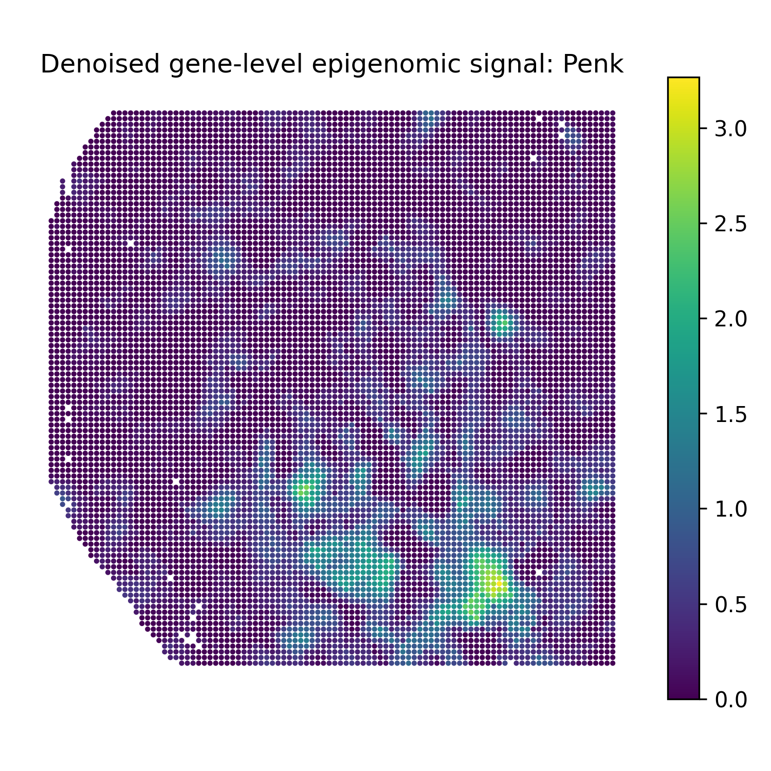
Gng2	Penk
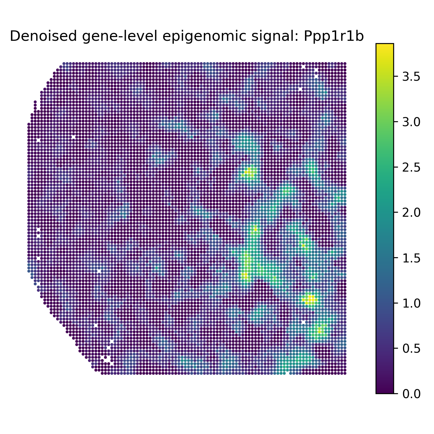
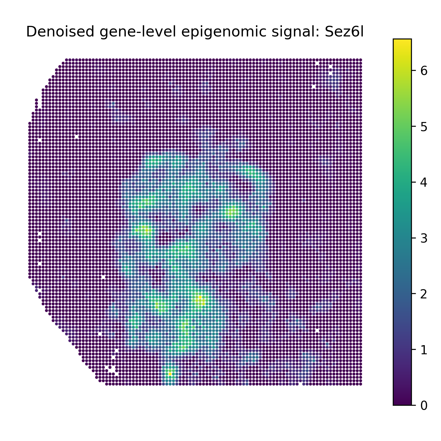
Ppp1r1b	Sez6l